In my current research, I am modeling consumer spending behavior to predict future income and spending. To do this I transform a set of transactions into a transaction stream, which is basically all the transactions for a given merchant or category (like ‘Gas Stations’). A conventional time series analysis is not appropriate since the series is not continuous and is irregularly spaced. These streams bear more similarity to Poisson processes and Weibull processes (under specific circumstances). The basis for the model is intermittent demand forecasting. Specifically there are methods that use bootstrapping to forecast the magnitude of future demand for a given window.
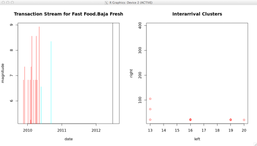
The biggest assumption with the bootstrap estimate is that events are IID, which in this case cannot be assumed. The reason is that this forecast is for a single individual, and people’s spending habits change over time. There are innumerable reasons for this: someone moves to a different city, they get a raise, they lose their job, they start dating someone, they go on a diet, etc. Hence a single transaction stream can have multiple regimes. If we are basing our forecast on a bootstrap, then the probability of an event occurring will be biased if the regime is ignored. In Figure 1 the probability of an event is 0.0144. However, most of the events occurred back in 2010, and there haven’t been any transactions at Baja Fresh since Q3 2010. Consequently the forecast will have a significant positive bias based on history that is no longer relevant. If we look at the two regimes (red, blue) the blue regime is active and an event occurring in this regime has a probability of 0.0026, which is a full order of magnitude less frequent.
Figure 1: Baja Fresh spending regimes
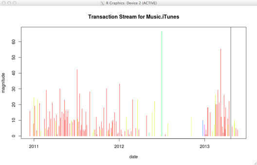
Another example of identifying distinct regimes is in Figure 2. In this case there are three regimes identified, where the red regime has returned after a hiatus. Clearly there is more spending activity in the red regime than in the green or blue regimes so including the green and blue regimes would produce a negative bias on the forecast transactions.
Figure 2: iTunes spending regimes
These spending regimes are identified by analyzing the interarrival times of the transactions. This is transformed into a two dimensional measure, which is on the right-hand plot. I then feed this into a standard agglomerative clustering approach with hclust. The key in this output is that the clusters are contiguous regions in the actual spending data. A naive clustering approach would not recognize the time dependence and would divide the transaction stream into disconnected slices that provide no useful information as shown in Figure 3.
Figure 3: Naive clustering of iTunes spending
Hence the key insight is that spending data has a time dependence associated with it and the analysis method needs to preserve that dependence. The simplest way of accomplishing that is by transforming the data into a form that preserves the dependence. This is no different from taking the log of a sequence of numbers to transform it into a linear problem.


I hate to ask, but I’m gonna anyway–any chance you’d be willing to turn this into a tutorial using R? And did you use the forecast library for the intermittent demand part, or something else?
LikeLike
I’m working on writing an article for these results. Once I do that I will discuss the implementation in more detail.
Regarding the intermittent demand part, no I didn’t use the forecast package. That only includes Croston’s method, which has known limitations. I also wasn’t satisfied with the results of the improvements to Croston’s method, including Syntetos-Boylan, etc. See the link to the Smart paper in the post. This uses bootstrapping as an alternative approach to Croston’s method.
LikeLike
Brian, I’m also interested in this problem and how you calculate your 2-dim. measure based on interarrival times. Can you provide a time-frame when your article will be available or at least a hint how you are doing this?
Thanks much!
LikeLike
I’m hoping to publish something in the coming months. I may just dump it on arxiv or ssrn. Before I discuss it in more detail I am running it through some simulated scenarios to test the accuracy of the regime detection. There is also a chance that it can be used for other applications as well.
LikeLike
Pingback: Para compensar meu silêncio… | De Gustibus Non Est Disputandum
Hi, Brian, say, can you give a status update on publishing your work on regime change in irregular time series? I”m really looking forward to taking a look at your methodology that you posted about back in July.
Thanks,
LikeLike
On the list of priorities 🙂 I actually have done some simulations to test the general accuracy, which has been very encouraging. I need to find a journal to publish the results. If you have any suggestions, I’m all ears.
LikeLike
Pingback: Lambda.r at FP Days 2013 in Cambridge, UK | Cartesian Faith