This is a lecture post for my students in the CUNY MS Data Analytics program. In this series of lectures I discuss mathematical concepts from different perspectives. The goal is to ask questions and challenge standard ways of thinking about what are generally considered basic concepts. Consequently these lectures will not always be as rigorous as they could be.

Solution sets for systems of linear equations

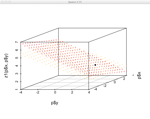
Let’s look first at a simple system of linear equations with a single solution. This system is from Example 1.10.1 of Kuttler.

What is this system telling us? If there is a unique solution, then we know that there is exactly one set of variables that satisfies all the equations. In addition, we know that all of the variables are independent. For our system above the solution is , which can be graphed using the R code below. Note that each equation is rewritten in terms of z.

z1 <- function(x,y) 25/6 - 1/6 * x - 1/2 * y
z2 <- function(x,y) 58/14 - 1/7 * x - 1/2 * y
z3 <- function(x,y) 19/5 - 2/5 * y

domain <- seq(-4,4, .5)
p <- expand.grid(x=domain, y=domain, KEEP.OUT.ATTRS = FALSE)
sp <- scatterplot3d(p$y, p$x, z1(p$x,p$y), pch=20, cex.symbols=.2, color='brown')
sp$points3d(p$y, p$x, z2(p$x,p$y), pch=20, cex=.2, col='red')
sp$points3d(p$y, p$x, z3(p$x,p$y), pch=20, cex=.2, col='orange')
sp$points3d(2,1,3, pch=20)

What happens if only two of the three equations are defined? This turns out to be quite interesting as the solution set becomes a line. The fact that the solution set is a line also tells us that the variables are no longer independent.

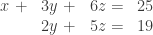
Let’s redraw our graph with only these two functions, along with the new solution set.

sp <- scatterplot3d(p$y, p$x, z1(p$x,p$y), pch=20, cex.symbols=.2, color='brown')
sp$points3d(p$y, p$x, z3(p$x,p$y), pch=20, cex=.2, col='orange')

sol <- function(z) data.frame(y=19/2 - 5/2 * z, x=-7/2 + 3/2 * z, z=z)
sp$points3d(sol(seq(-4,7,0.5)), type='l')
sp$points3d(2,1,3, pch=20)

As a bonus, I drew the original solution when we had three functions. Thankfully this point is contained within the larger solution set. Going in the opposite direction, if we start with a single equation, our solution set is a plane. Adding a second equation to the system yields a line, and a third equation yields a point. If we consider these equations as constraints in an optimization problem, it is easy to see how additional constraints can reduce the solution set.

Notice that we arrived at this solution set by using only two of the three equations. Sometimes a system with three equations can result in a non-unique solution because the equations are not dependent. In Example 1.10.4 of Kuttler, the following system of linear equations is listed.

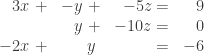
Solving this system leads to the same situation, where the variables are dependent.

Exercises

• Use the sol function to verify that our unique solution {1,2,3} is a member of the line
• Graph the solution set for equations 1 and 2
• Write the function for the solution set of 1.10.4 and graph its result

Linear transformations

In the previous section we looked at systems of linear equations. Each equation can be considered a function in two variables. Since these are linear equations, our solutions are (hyper) planes. What if instead of solving for a specific solution that satisfies each function, we use a matrix to represent a function that changes a set of values? These are linear transformations and are quite common. Anyone that has created a score or measure from a weighted set of variables has applied a linear transformation. The definition of a linear transformation (2.19 of Kuttler) is simply a restatement of the properties of linearity for vectors instead of scalars. This is easier to understand by rewriting as a function . Then we get .

The simplest linear transformations are for matrices that are simply a row vector. As an example suppose we want to model which twitter users are the most internet savvy based on their usage stats. We define this as . Our transformation matrix is then . Given a user u, their internet savviness is just . Knowing what we know about matrices, we can construct a matrix with all users and calculate their savviness measure in a single operation. We’ll use a data file of tweet information that looks like

> head(z)
                      created_at
1 Mon Dec 02 23:35:49 +0000 2013
2 Mon Dec 02 23:35:48 +0000 2013
3 Mon Dec 02 23:35:48 +0000 2013
4 Mon Dec 02 23:35:47 +0000 2013
5 Mon Dec 02 23:35:46 +0000 2013
6 Mon Dec 02 23:35:45 +0000 2013
                                                                                                                                          text
1 RT @Citizenship4All: Fasters, families pray outside of @SpeakerBoehner's office: May Congress realize "they are servants of the people." ht&
2 RT @msnbc: What is the most important issue Congress should act on before they head home on December 13? Take our poll: http://t.co/VIHjzbc&
3 RT @EWTN: Argentine congress recommends Pope Francis for Nobel Peace Prize: Buenos Aires, Argentina, Dec 2, 2013 / 05:55... http://t.co/2Ts&
4 RT @Scalplock: ACTION: Congress Likely to Vote on Gun Control Today. Dec 2.  http://t.co/78JLTdcPMb Schumer worked overtime during Thanksgi&
5                                          Americans Want Congress Members To Pee In Cups To Prove They're Not On Drugs http://t.co/LVSHu2b0iI
6     Vote for @politifact's lie of the year! I voted for @SenTedCruz's "Congress is exempt from #ObamaCare" lie here - http://t.co/r4rPv8Ns6W
  retweet_count favorite_count user.screen_name user.followers_count
1            16              0   HutchissonMike                  617
2             1              0       srwrdm1221                   68
3             1              0     sistervpaul_                  616
4             1              0     anthonydiana                 1567
5             0              0          linmom1                    1
6             0              0  DigitalMaxToday                  972
  user.friends_count                user.created_at user.favourites_count
1               1345 Tue Apr 23 14:29:36 +0000 2013                 11179
2                553 Sun Jul 21 11:58:49 +0000 2013                    14
3                643 Fri Sep 06 18:42:40 +0000 2013                  3495
4                968 Fri Jul 24 22:42:20 +0000 2009                  4136
5                  1 Tue Oct 13 02:36:08 +0000 2009                     0
6               1362 Wed Feb 22 00:32:24 +0000 2012                   605

(When I get a chance I will post the file so people can try out their own measures.)

z <- read.csv('~/congress.csv', as.is=TRUE)
u <- as.matrix(z[,c('user.followers_count','user.friends_count',
  'user.favourites_count')])
A <- as.matrix(c(3,1,2),nrow=1)
A %*% t(u)

Using this example as a starting point, what does it mean for to have multiple rows? Additional rows are merely additional aggregate measures. Consider a measure for receptiveness, which we define as the amount someone is willing to retweet someone else’s post. What variables might go into a measure like this? As a naive first try how about favorite/day, and friends/followers. To calculate averages on a daily basis we want to determine the age of an account and bind this to our matrix.

age <- Sys.Date() - as.Date(z$user.created_at, format='%a %b %d %H:%M:%S %z %Y')
u <- cbind(u, favorites=u[,'user.favourites_count'] / as.numeric(age))

Note that this gives us a different set of variables from the first measure. At first glance this may seem problematic, but since this is a simple linear combination all that needs to be done is to union the variables and set the irrelevant ones to 0. Hence we can update A to be A <- cbind(A, 0).

This lesson provides some perspectives on matrices and how to apply them to the analysis process. Obviously matrices and linear algebra have a wealth of applications, so these are not the only interpretations. The goal here is to provide you with tools for how to conceptualize their usage. As we progress through the course, we will explore other interpretations of matrices along with their application. One point to consider is how here we are explicitly building a function to transform data, whereas in the previous section we were trying to find a solution to a given set of functions. In a later lecture, we will compare and contrast this approach to a linear regression.

Exercises

• Update the savviness measure to normalize friends and followers based on age of account
• Create the receptiveness measure and update the u and A matrices